Imaging geological thin sections
Table of contents
Overview
Geological thin sections are specimens of geological material which are thin enough to be mounted on microscope slides.
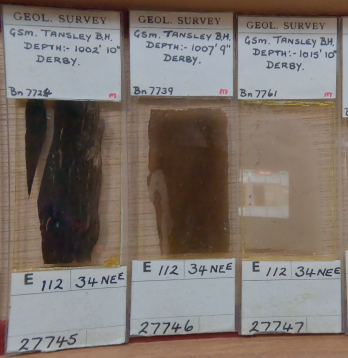
Figure 1: Example of three example thin section slides. Taken with kind permission of the BGS.
Roughly 30 microns thick, these sections are semi-transparent allows them to be viewed under a microscope which reveals how they are constructed. The use of polarising filters allows more information on the structural and chemical makeup of geological specimen to be obtained.
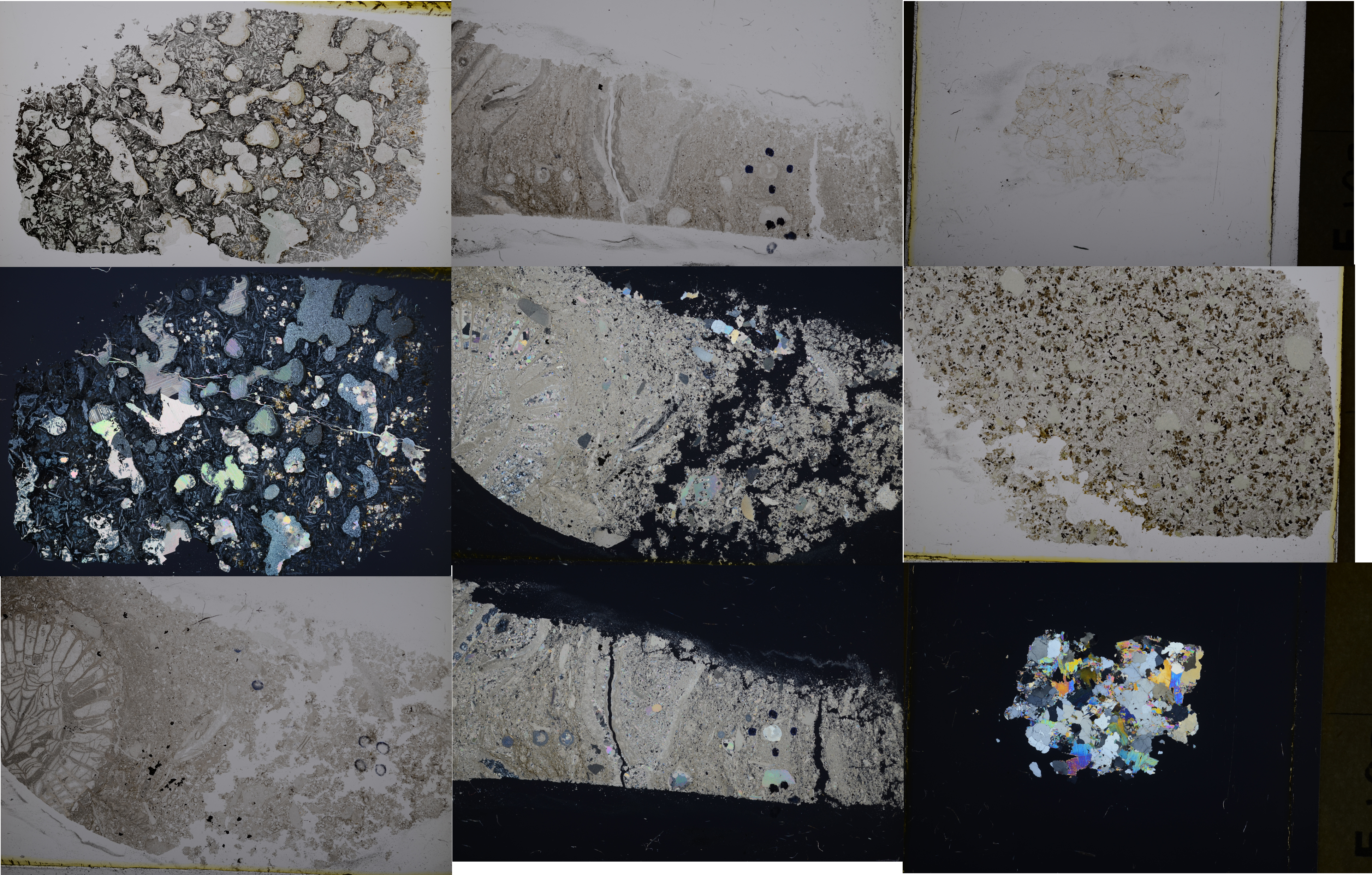
Figure 2: A selection of thin section images taken using this workflow. Taken with kind permission of the BGS.
Video
The video below shows the imaging workflow used by the British Geological Survey to image their slide collection.
Workflow
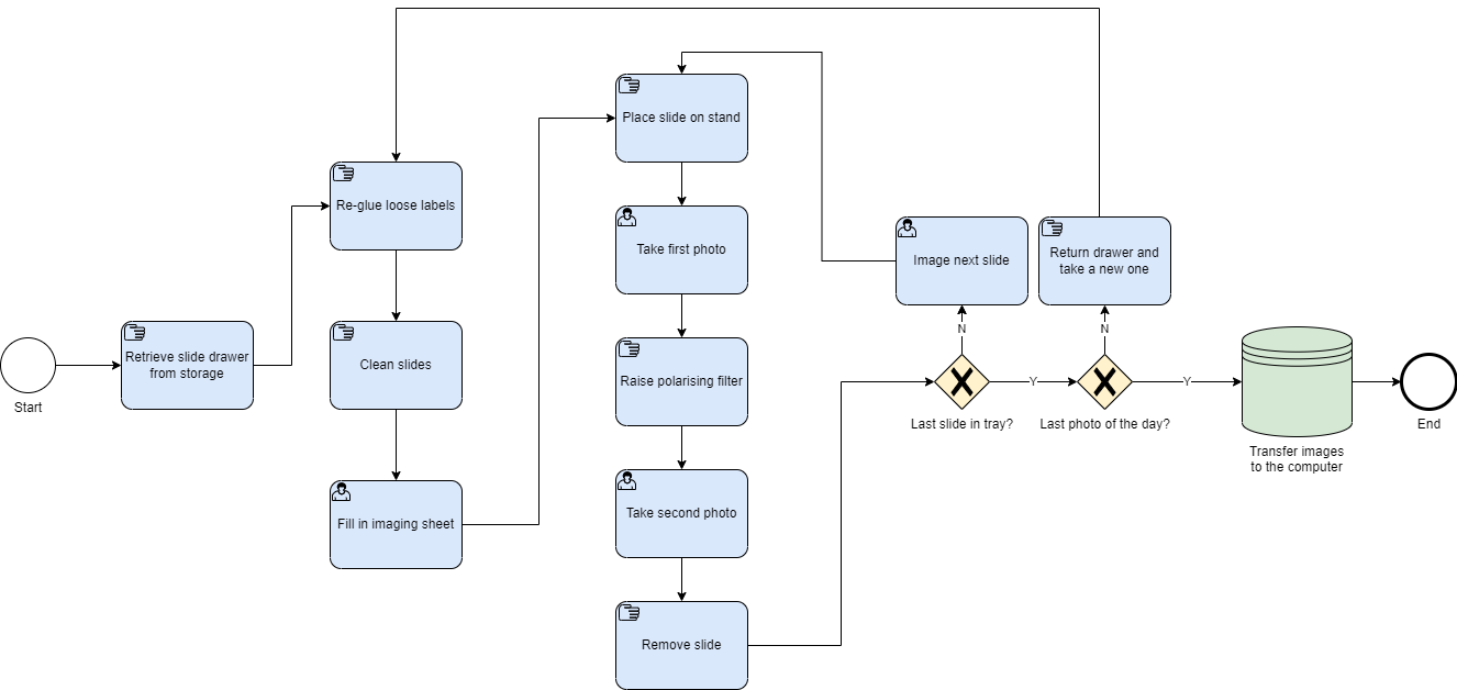 Figure 3: Workflow diagram of decisions and steps for the imaging of geological thin sections.
Here we present an overview of the imaging workflow which has been used to digitise the majority of the British Geological Survey’s (BGS) thin section slide collection. This workflow has been highly effective in producing quality images of thin section specimens, and is highly efficient being capable of producing images on over 1000 specimens a day.
Pre-Digitisation Curation
Thin section slides were housed in drawers like this:
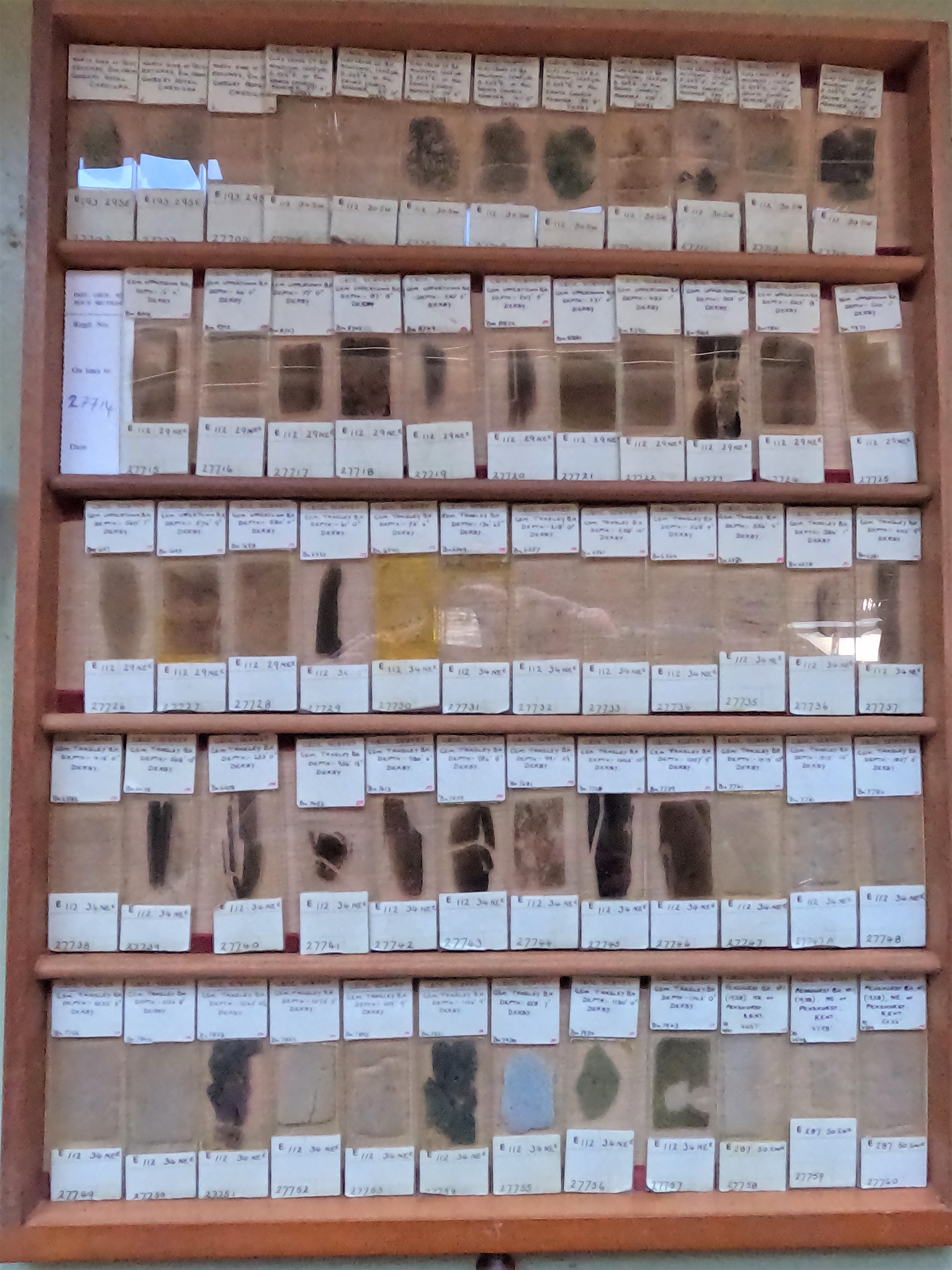
Figure 4: Drawer of thin section slides. Taken with kind permission of the BGS.
There are several steps that need to be performed to ensure that the specimens are ready for imaging which will also help the curation and preservation of your specimens. The steps that need to be taken in this section are:
-
Labels - some labels may be loose and need to be reattached. We reattach labels to their slides using a small amount of pH neutral PVA glue, applied using a cocktail stick. Press the label down and leave to dry. Check all slides to ensure that labels are attached.
-
Slide cleaning - glass slides stored for extended periods of time are likely to be dusty and dirty. This can obscure the specimen images. To clean slides, they are treated with a moist square of paper towel sprayed with sensitive skin dish washing detergent mixed in RO water in a 30:70 mix. Take each slide in turn and rub with the paper towel, the cleaning action is similar to that of cleaning glasses. Watch out for broken slide and loose coverslips. Labels should be written in waterproof ink, but avoid these areas if the specimen just incase.
-
Specimen ordering - in our system, thin section specimens have a unique identifier within each tray (e.g. E1, E2, E3, E4 etc). We order the tray in alphanumeric order. If there is a missing slide number, a gap is left. This ordering helps organise the imaging process.
Image Capture
- Imaging set up
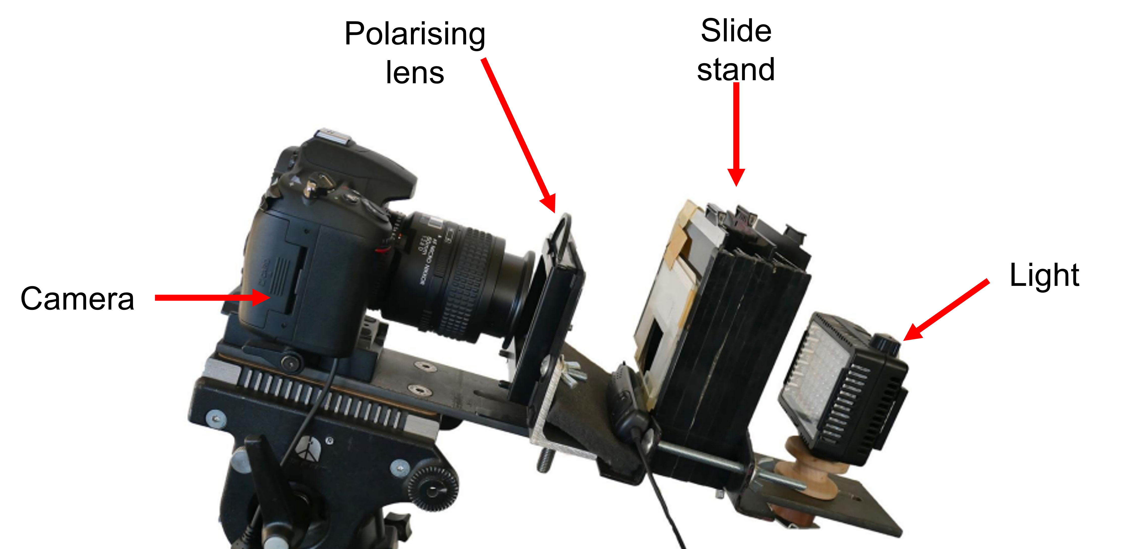
Figure 5: Annotated diagram of the set up. The downwards angle keeps the slide in place. Taken with kind permission of the BGS.
The imaging set up is composed of:
- a DSLR camera
- a removable polarising lens
- a slide stand on which the slide specimens sit. This also contains a second polarising lens and a piece of translucent Perspex which flattens the light from behind.
- a light source. Illuminates the slide from below, similar to a microscope does. All components are attached to metal beam which keeps all components lined up in a straight line. This beam is angled downwards which prevents the specimen from falling out when placed on the stand.
- Imaging process
To image, we place the slide at the front of the slide stand. We position the slide so that the sample is centered and can be seen by the camera. The angled set up will keep the slide in place. We then take the images. Two images are taken.
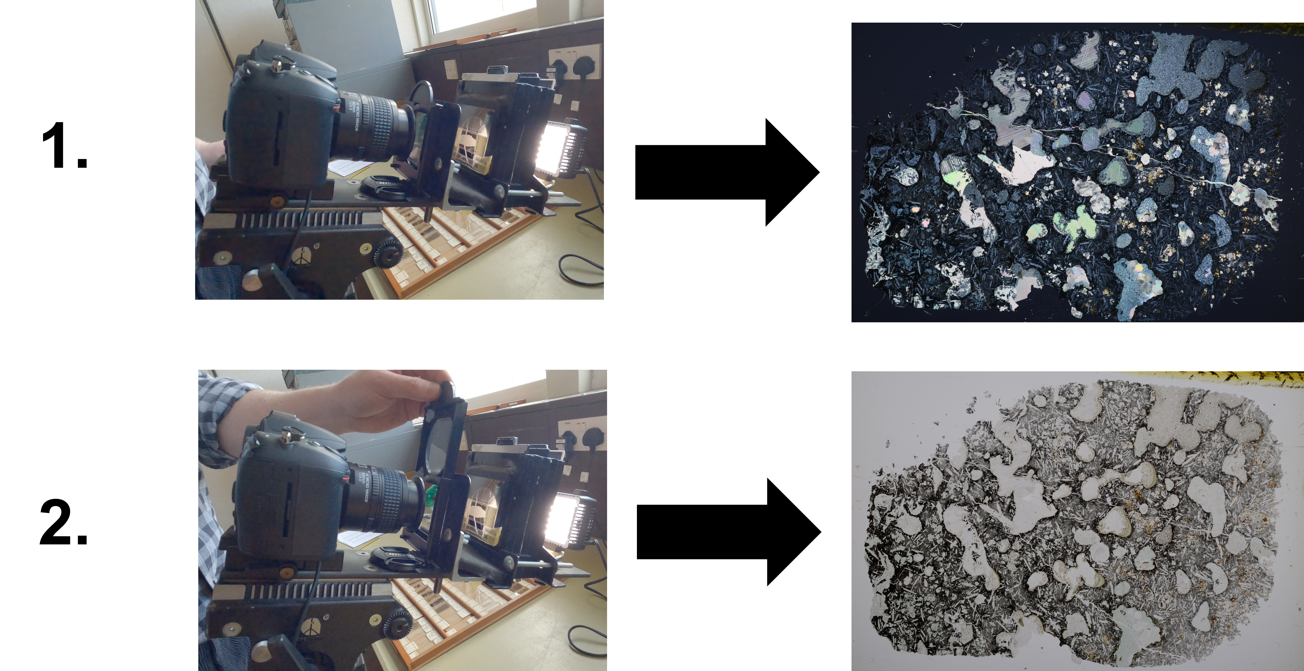
Figure 6: Diagram of the order of taking the two images showing the filter position and an example image of each. Taken with kind permission of the BGS.
The first image is taken with the removable polarising lens down. The polarised light creates a darker image where some structural features are more distinguishable. The image is taken using the connected remote shutter button. The camera makes a click as the image is taken and after a second it appears on the camera’s LCD screen. We check this screen to make sure the photo has been taken correctly.
For the first image, write down the image number on the recording sheet (further details below).
Once the first image is taken, the removable polarising lens is lifted and a second image is taken. This image produced is lighter in shade than the previous one. After checking that it appears on the screen correctly, the slide is removed and returned to the tray. The process is repeated for the next slide.
Once the last slide in a tray has been imaged, we check that the number of photos taken is two times the number of slides in the drawer. The final image number should also be 2 times the number of slides plus the first image number. If correct, the drawer is returned and a new one is taken. The process then begins again.
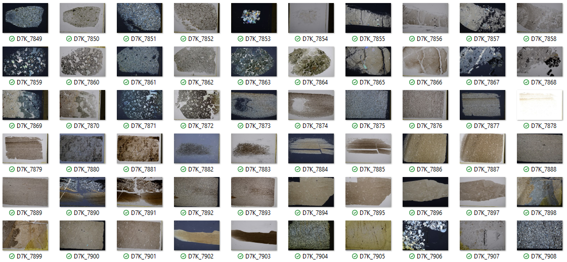 Figure 7: A collection of thin section images after being downloaded from the camera’s memory card.
Image Processing
Image files are downloaded from the camera’s memory card. Images are then matched to their record using the image and section number.
Image correction processing was carried out in Photoshop.
Images were also converted to the JPEG2 format.
Electronic Data Capture
This sheet records data about the specimens and their images, and creates a link between the two so that records can be created.
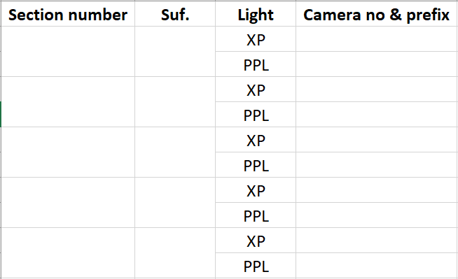
Figure 8: A focused example of a blank recording sheet. Reproduced with kind permission of the BGS.
We fill in the columns as follows:
- The Section number column is the unique number the slide is given in the collection (e.g. E27746, E27747 etc).
- The Suf. column is for section numbers that include extra notation. Sometimes two slides have been created from the sample and thereby have the same section number, but are differentiated by their suffix (e.g. E27747 and E27747A).
- The Light column is either XL for the first image where the filter is down (double polarised light), or PPL for the second image where the filter is up (plane polarised light).
- In the Camera number & prefix column we record the image number as assigned by the camera. These will be filled in in a series on after the other. If a mistake is made, we leave the image in the camera and miss out that number in the column. See the image below for an example (the number 7853 is missed out). It is important to make sure that this column is filled in correctly. Any mistake will result in the wrong image being attached to each specimen.
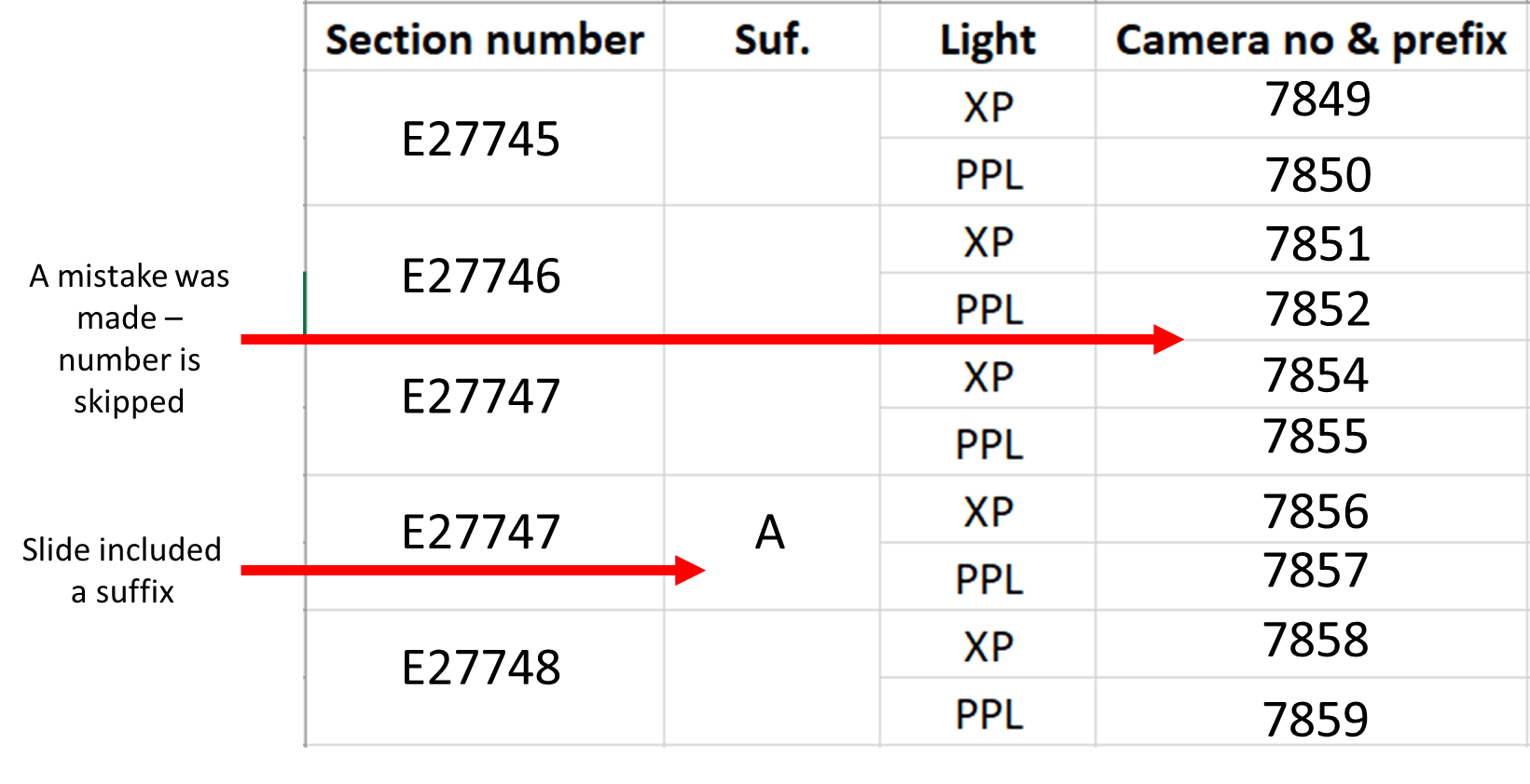
Figure 9: A focused example of a completed recording sheet with annotations. Reproduced with kind permission of the BGS.
In practice these details were recorded on paper sheets and entered into excel later, but could in principle be directly entered into a spreadsheet.
Preserving and Publishing Data
Images taken with this workflow have been uploaded to the BGS’s online repository and are available for free to the public.
Images are available from the BGS Britrocks website.
Further developments and plans
While this workflow has proved successful when used in-situ at the BGS headquarters in Keyworth, a number of changes are being developed to both improve the process and to make this workflow usable for digitisation efforts at other collections.
- Barcodes - barcodes were not used initially in this project. However, unique barcodes attached to specimens allow individual specimens to be identified accurately and easily.
Unique identifier barcodes have become the standard in digitisation and have been utilised for many different specimen types. Barcodes can link specimens to digital records more easily and with fewer potential mistakes than the recording approach used here. The use of multiple barcodes, such as that used in this workflow for microscope slides at the NHM illustrates that a series of barcodes can even be used to create digital records for specimens automatically.
Attaching barcodes to thin section slides would appear like this:
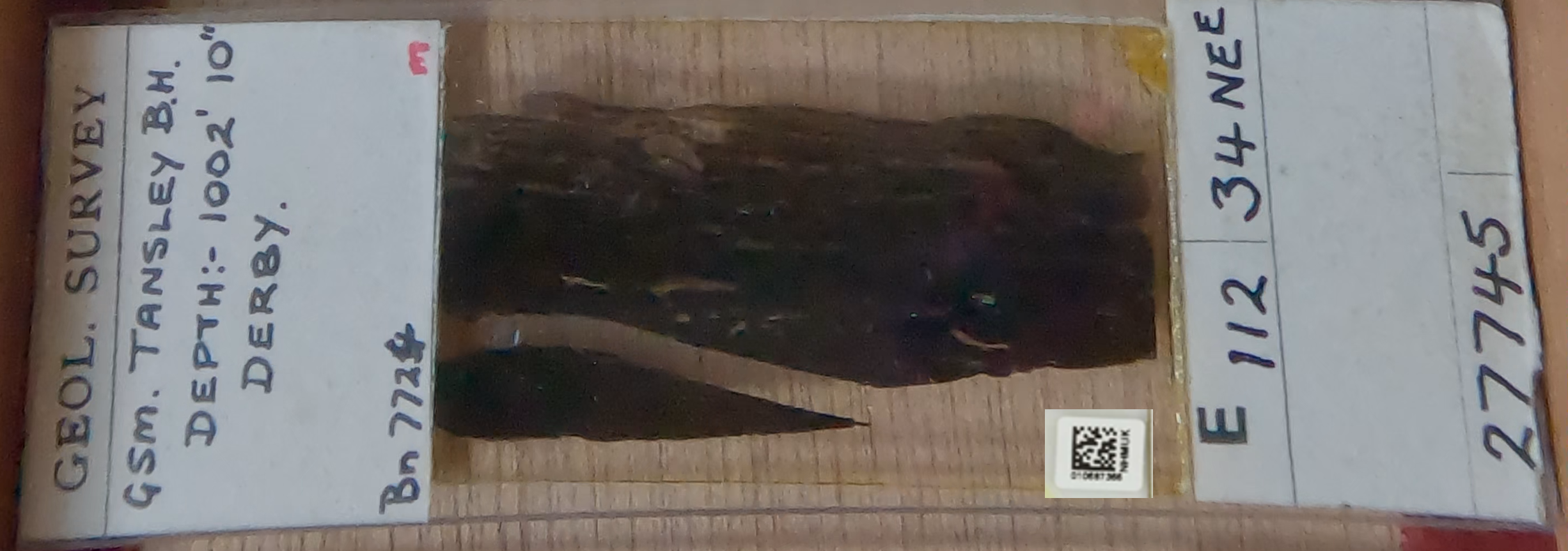
Figure 10: Thin section slide with barcode. The barcode is unique to this specimen and can be read with a scanner or bar code reading software from a specimen image. The barcode does not cover any of the specimen.
- 3D printed components - the original imaging set up was designed using available parts that were already available at the BGS. While this was successful for this project, replication of these precise components would be difficult for others.
To solve this issue, alternative components have been designed using the software Openscad. These components can be 3D printed to produce a replicated imaging set up.
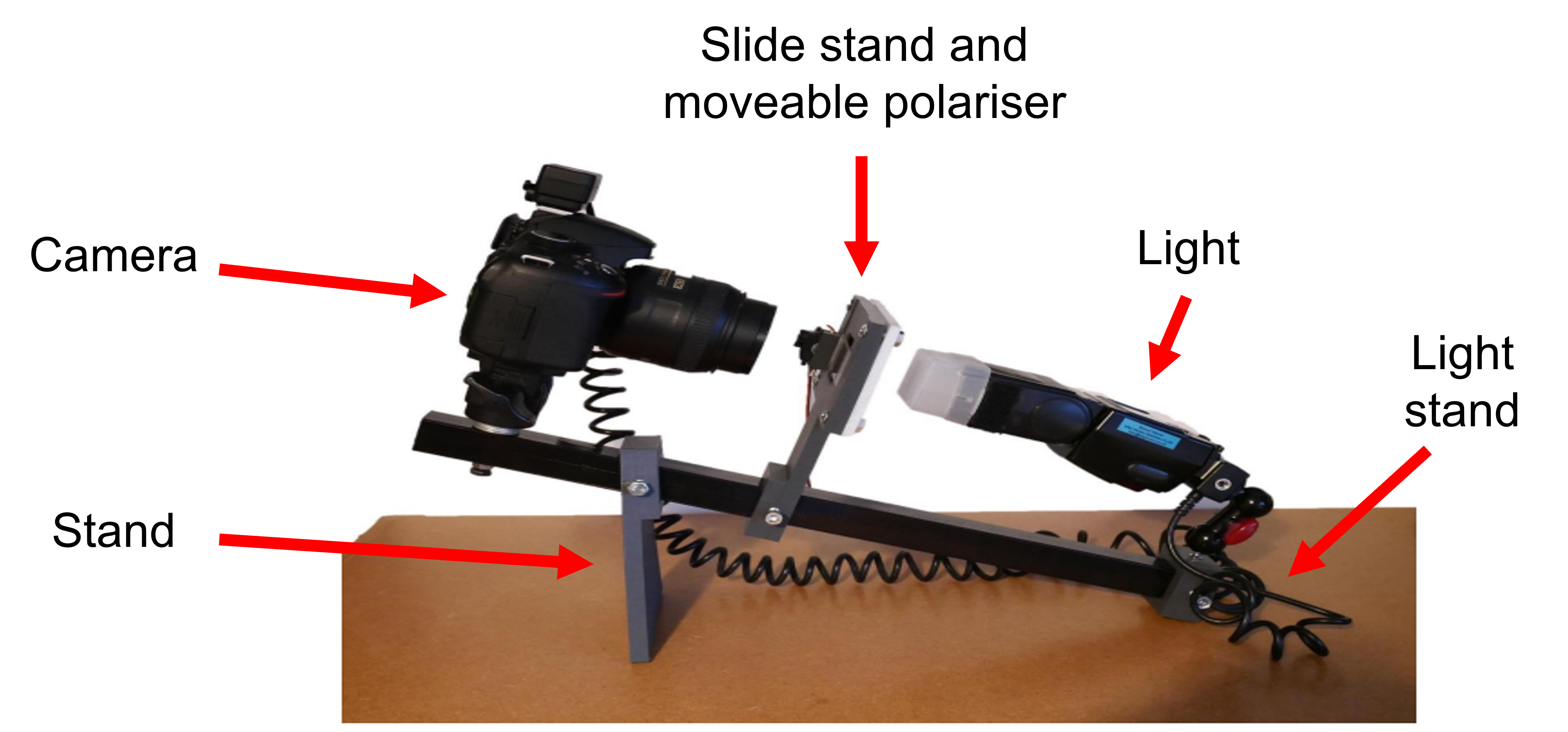
Figure 11: Annotated set up using 3D printed parts. The 3D printed parts are a stand to create the angle of te set up, a slide stand which includes moveable polarising filter, and a light stand to which the light can be fixed to. All are deigned to fix around a squate shaped metal rod.
This set up is fixed to a metal bar and would have the camera at one end. Components are fairly cheap to print and can be easily assembled. A prototype has already been produced and produces quality images or thin section slides.
The files of the 3D components are availiable from our GitHub repository.
- Image automisation - in the current set up, the polarising filter must be raised in between the two photos of a single image. Although this doesn’t take too much time, it is another physical step to be completed. It can lead to occasional photo errors when the filter is not raised completely, and physical contact with the set up which can affect the image.
A better solution would be to automate the process with one action which would take both images. This has been piloted using a small motor and controlled by a small single board programable computer such as a Raspberry Pi or Arduino. This would move the filter between shots without the need to move it manually and also take both images.
An example of this can be seen here. This was programmed using the code found here.
- Image processing - image processing is currently perfomed manually in Adobe photoshop. This is a liscened program with a fee. We are developing an alternative process using free software such as Image magick which would make the processing of images feasible for more collections. The process could also be automated using hot folders so that all imported images are processed in the same manner.
Example Projects
This workflow was used to digitise the BGS’s whole thin section collection as part of their Britrocks project
Requirements
Hardware
The workflow presented here uses:
- Camera - above used a Nikon D7000
- Lens - 60mm f2.8 Micro
- Polarising filter x2
- Light source - Godox LED video light (Model:LED 64)
- Translucent Perspex sheet
- Stand for slides - made of stack of double dark slides (one polarising filter and Perspex sheet are imbedded into the slide stand).
- Remote shutter button
- Camera tripod - topped with a monopod head with quickrelease.
- Metal beam - to attach components to.
Future requirements may include:
- 3D printed components
- Rasberry Pi / Arduino
- servo motor
Software
Microsoft Excel Adobe Photoshop
Future requirements may include:
- Openscad - for 3D printing of components.
- Image magick - for automated image processing.
- Code for moving filter
Camera Settings
The camera is set to ‘aperture priority’. With no slide present this results settings of:
- Aperture = F8
- Shutter speed = 1/2
- ISO = 200
Images are saved from the camera in the JPEG format.
Resources
Digitisation Rates
The estimated digitisation rate for this workflow is 1 minute per slide (including image capture and image processing). This assumes the collection has already been organised and the pre-digitisation curation step is complete.
For one tray of 60 slides (shown in the video), we estimate the image capture stage will take roughly 30 minutes:
- Remove tray and appraise – 5 minutes
- Generate list of samples in trays, complete with spaces to record XP and PPL images – 5 minutes
- Photograph 5 lines of 12 slides and record numbers – 10 minutes
- Ensure slides are back in tray, sort out any problems like loose labels – 5 minutes
- Break – 5 minutes
During the BritRocks project, the image processing step would be completed once there was a batch of 10,000 images (5000 slides). This would take roughly a full day to complete, and would include:
- Splitting images into plane polarised (PPL) and cross polarised (XL) light
- Checking there are the same number of PPL and XL images
- Checking images are correct – all PPL images should be pale, XP should be dark
- Basic batch image processing in Photoshop
- Linking images to the database using a join query against specimen number
- Spot checks of images against slides to check the linking is correct
- Converting to JP2 files and transering files to corporate server Many of these steps will be dependent on an institution’s IT infrastructure (e.g. collections management system, software available to do batch image processing), and therefore the rates may vary.
Other Sources
Blog posts recording the progress of project:
100,000 Scottish thin sections completed!
BGS thin sections: 150,000th image taken!
Authors
Michael Jardine (Natural History Museum), Simon Harris (British Geological Survey)


Contributors
Bob McIntosh (BGS Edinburgh)
References
British Geological Survey petrology collections in Geikie and the development of petrography, particularly in Scotland John R. Mendum and Michael P.A. Howe. Geological Society, London, Special Publications, 480, 367-377, 16 January 2019, https://doi.org/10.1144/SP480.19
Eberspächer, Susanne & Lange, Jan-Michael & Zaun, Jörg & Kehrer, Christin & Heide, Gerhard. (2015). The Historical Collection of Rock Thin Sections at the Technische Universität Bergakademie Freiberg and Evaluation of Digitization Methods. https://www.researchgate.net/publication/273118591
Haaland, MM, Czechowski, M, Carpentier, F, Lejay, M, Vandermeulen, B. Documenting archaeological thin sections in high‐resolution: A comparison of methods and discussion of applications. Geoarchaeology. 2019; 34: 100– 114. https://doi.org/10.1002/gea.2170
Licence
The content of this workflow is the property of the Trustees of the Natural History Museum and of DiSSCo UK, unless were otherwise stated. It may be used under a creative commons licence. Images and information have been kindly provided by the British Geological Survey (BGS).
Citation
Jardine, M.D. and Harris, S. (2022) DiSSCo Digitisation Guide: Imaging geological thin sections - BGS. version 1.3. Available at: https://dissco.github.io/Geo/thin_sections.html
Document Control
Version: 1.3
Changes since last version: Digitisation rates added
Last Updated: 15 September 2023
Edit This Page
You can suggest changes to this page on our GitHub